DistServe Part 1: Understanding Prefill, Decode, and Goodput in LLM Systems

DistServe is one of the most important papers for understanding the modern inference and LLM serving systems like NVIDIA Dynamo, vLLM, SGLang, etc. My goal with this is to provide a first principles understanding into the mechanics and optimization problem of LLM Serving for engineers and entry-level researchers alike.

Core Problem Formulation and Why It's Hard?

The paper starts on the assumption that we want to serve LLM requests while meeting SLO requirements for TTFT, and TPOT, while maximizing the goodput per GPU under realistic workloads. At its core, DistServe reframes LLM serving as a constrained optimization problem under dual latency SLOs.

I KNOW, I KNOW! That's too much to start off, and as promised we will build this from first principles. So before moving forward, there was a lot of technical jargon in this statement. So let's break down the basics:

SLO: Service Level Objective; a target your system promises to hit for some metric

TTFT: time-to-first token; basically the latency to first token

TPOT: time-per-output token; per-token latency during decoding

Goodput: max sustainable request rate while meeting SLO targets; throughput which meets system requirements

Throughput is the Wrong Metric

In LLM serving, raw throughput is a misleading metric. A system can process more requests per second while simultaneously degrading user experience if those requests violate latency SLOs. Thus, DistServe optimizes for goodput.

What DistServe optimizes for:

• maximizing goodput = the highest sustainable request rate such that:
• • TTFT SLO is met (e.g., p90 TTFT <= some bound)
  • TPOT SLO is met (e.g., p90 TPOT <= some bound

This is majorly an optimization problem under the dual latency constraints using a goodput objective.

Since we have now defined the optimization objective, let's talk about why is maximizing goodput under dual SLOs is a hard problem to solve.

Why is this (fundamentally) hard?

Although inference involves many small steps, its latency behavior is governed by two major computational regimes: prefill and decoding.

The Autoregressive Constraint

Modern large language models are autoregressive transformers. This means that at every step, the model predicts the next token conditioned only on the tokens that came before it. Attention is causal: token t can attend to tokens 1 through t − 1, but never to future tokens.

This causal structure has an important systems implication.

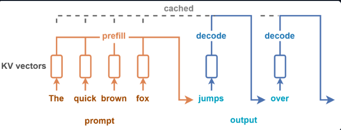
During the initial forward pass over the input prompt, the model computes key and value vectors for every token at every layer. These key–value pairs are stored in what is called the KV cache. The KV cache acts as a compact summary of the prompt’s contribution to future predictions.

When generating a new token, the model does not recompute the entire prefix. Instead, it computes a new query vector for the current token and attends to the previously stored keys and values. In other words, decoding depends only on the existing KV cache and the current token — not on re-running the full prompt.

This structural property creates a natural computational boundary: one phase builds the KV state, and the other consumes it incrementally. That boundary is what divides LLM inference into two distinct regimes: prefill and decode.

Phase A: Prefill (Prompt Processing)

In the prefill step of LLM inference, the model processes the entire input prompt in a single forward pass to initialize the autoregressive state. So during pre-fill:

• The transformer runs over all L_in prompt tokens
• For each layer, it computes and stores:
• • Key vectors
  • Value vectors
• These are stored in the KV cache, which summarizes the prompt for future decoding.
• Workload is dominated by:
• • Large matrix multiplications dominate.
  • Phase is compute-bound
• User-visible effect:
• • determines the TTFT, the model produces the first output token.
  • If prefill is delayed or slow, the model feels unresponsive.
• Intuition:
• • Prefill is a single large burst of work per request.
  • It is chunky, heavy, and sensitive to prompt length.

Phase B: Decode (token-by-token generation)

Decode is the incremental phase where the model generates output tokens one at a time using the previously computed KV cache. During decode:

• For each new token:
• • The model computes a query vector
  • That query reads/writes from all the previous stored keys in the KV Cache
• Only the new token’s computation is performed.
• Cost per step grows (linearly, why?) with current context length (more tokens in cache to attend over)
• Workload is dominated by:
• • KV cache reads
  • Smaller matrix multiplications
  • Phase is memory-bandwidth-bound
• User-visible effect:
• • determines the TPOT
  • If decode is delayed or uneven, the stream feels choppy or stalled.
• Intuition:
• • Decode is many small, repeated jobs.
  • It requires steady scheduling cadence to feel smooth.

Key asymmetry:

• Prefill is a “chunky, heavy job” (big burst of work); cost ~ Σ Lᵢ² (in detail in next part)
• Decode is a “many small jobs” (steady cadence) ~ λ · E[L_out] (in detail in next part)

Because decode workload scales with λ · E[L_out] while prefill scales with λ, increasing traffic stresses decode disproportionately.

This difference is where the scheduling pain comes from.

Setting the naive baseline

We start by putting prefill and decode on the same GPUs, and they share the same scheduler and batch to keep GPUs busy.

Here's what would happen in a simple queue on one server:

• Prefill: let's assume each job would take a service time close to 100ms (due to big chunks)
• Decode: service time = 5ms due to tiny steps but repeated multiple times during one request

Let's say you mix them up in one FIFO queue: when a prefill job starts, for the 100ms, all the decode jobs wait behind it, even though each need only 5ms. That waiting time would directly inflate the TPOT (tokens pause streaming).

Let's say instead multiple decode jobs are queued up before the prefill job, the first token output has to wait longer until the decode steps are complete. This inflates the TTFT metric.

This is the fundamental conflict:

• TTFT wants “start prefill quickly”
• TPOT wants “never stall decode steps”
• a single shared queue cannot satisfy both well at high load

Again, Batching is usually good for throughput in general, but under two-phase workloads it can hurt:

• Prefill batching: great GPU efficiency, but it creates large “prefill blocks” that can delay decode.
• Decode batching: improves efficiency per step, but you must schedule steps frequently to keep streaming smooth.

So “batch better” doesn’t eliminate the underlying conflict; it just shifts where it shows up. This is not a scheduling bug. It is a structural conflict between two incompatible latency objectives.

Separating the Incompatible

I am hoping that you are with me until here. The understanding that you need to develop here is one on the basis of intuitiveness. We now have two workloads with opposite preferences: prefill wants large, compute-heavy batches; decode wants small, latency-sensitive steps. Any shared scheduler must compromise between them and under high load, one SLO will inevitably fail first.

At that point, the question shifts. Instead of asking how to schedule them better, we must ask a more fundamental question: why are we scheduling them together at all?

Why Prefill and Decode Can Be Separated

Let’s reason from first principles. In a transformer:

At decoding step t, the model needs:

• The current token embedding.
• The model weights.
• The KV cache for all previous tokens.

That’s it.

Formally:

$h_t=TransformerStep(x_t,K{V}_{1:t-1})$

So the prefill computes:

$K{V}_{1:L_{in}}$

and produces the first output token y_1, then decoding can continue independently from that state.

This is the key structural property:

The KV cache is a sufficient statistic for continuing generation.

Nothing else from prefill is required. That makes the argument for architectural split valid.

Why Separation Helps

Prefill and decode stress different parts of the hardware.

Prefill is dominated by large matrix multiplications over the full prompt. It is compute-bound, benefits from large batched GEMMs, and its primary objective is minimizing TTFT.

Decode, by contrast, generates tokens incrementally. Each step reads from the KV cache and performs smaller matrix operations. It is often memory-bandwidth-bound, sensitive to scheduling cadence, and its objective is minimizing TPOT.

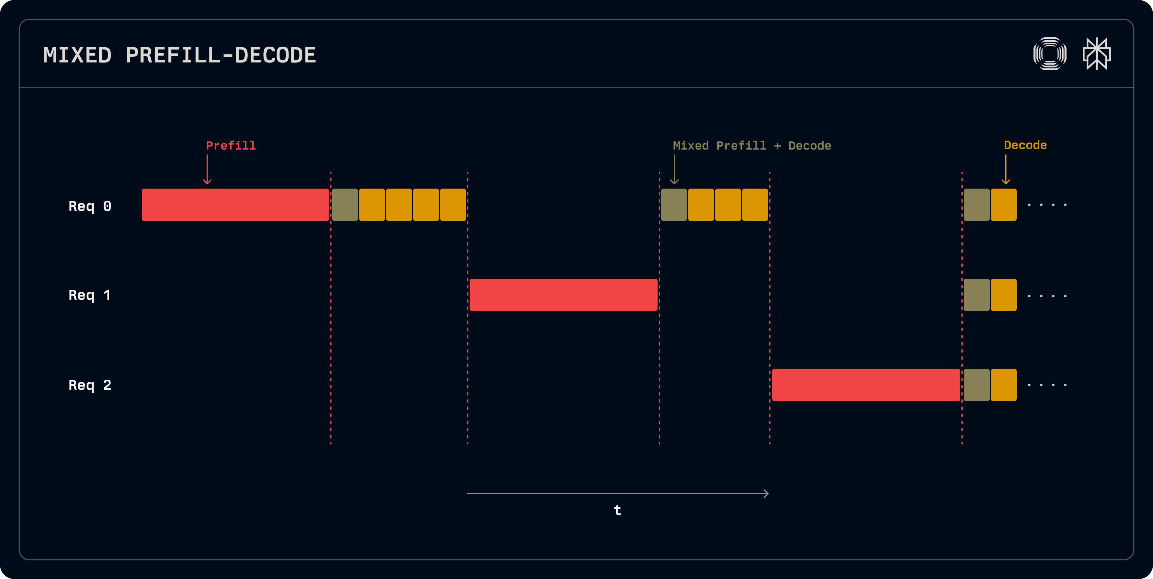
When colocated on the same GPU pool, these two workloads interfere:

• Large prefill bursts stall decode steps.
• Frequent decode steps delay new prefill jobs.
• Parallelism and batching strategies must be shared.

This forces a compromise between incompatible optimization goals.

Disaggregation removes that compromise.

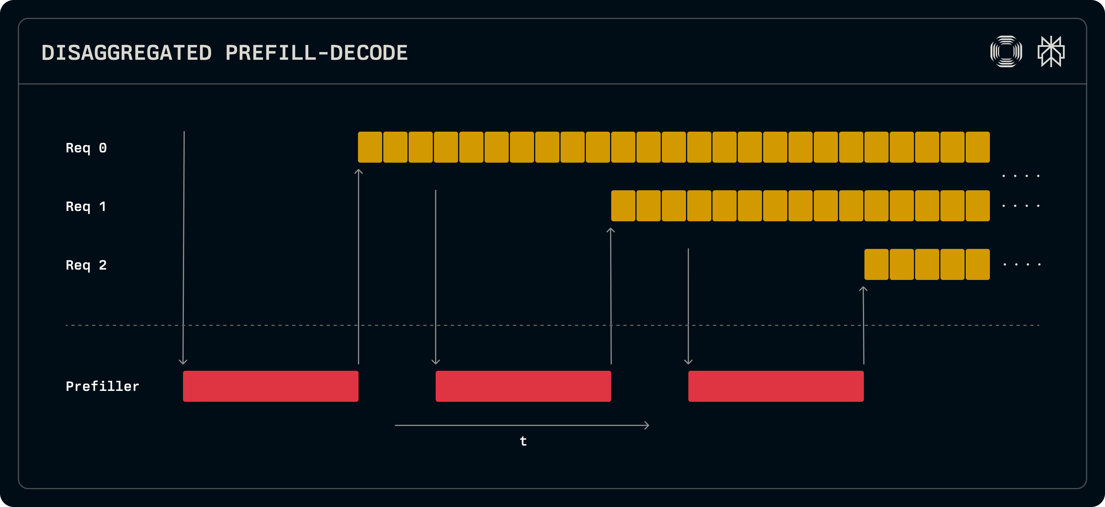
By separating prefill and decode into distinct GPU pools, we decouple:

• Queues
• Parallelism strategies
• GPU allocation

Now each phase can be optimized independently and the problem becomes one of resource allocation: how many GPUs and what parallelism should each pool use so that neither TTFT nor TPOT becomes the bottleneck?

That allocation problem is the core systems challenge.

DistServe Architecture

Let’s describe what happens when a request arrives.

Step 1 — Router

The request hits a front-end router.

The router:

• Sends the request to a prefill GPU pool.
• Does not send it to decode yet.

Important: prefill and decode are physically separated pools.

Step 2 — Prefill Pool

On the prefill GPUs:

• The system batches multiple prompts.
• Runs full transformer forward pass over each prompt.
• Produces:
• • First output token
  • Full KV cache for each layer

Now TTFT is determined by:

• Queue delay in prefill pool
• Prefill compute time

Decode has not started yet.

Step 3 — KV Handoff

The KV cache is transferred from:

• Prefill GPUs
  to
  
• Decode GPUs

This may be:

• Intra-node (NVLink, fast)
• Inter-node (network, slower)

This is the new cost introduced by disaggregation.

Step 4 — Decode Pool

Decode GPUs:

• Maintain their own queue.
• Batch token steps across multiple requests.
• Run incremental forward passes:
• • 1 token at a time
  • Using KV cache

TPOT is determined by:

• Queue delay in decode pool
• Per-token compute time

Prefill no longer interferes.

Final Thoughts

So far, we focused on the structural insight: LLM inference is governed by two fundamentally different computational regimes, and colocating them creates unavoidable interference under dual SLO constraints. We also discussed the fact that we separation helps, and a brief introduction into the DistServe architecture.

For now, we have reasoned at the level of structure and intuition. We have NOT YET formalized the latency scaling laws, nor have we derived the optimization procedure required to maximize goodput. But once prefill and decode are separated, a new question emerges: how do we allocate GPUs and configure parallelism to maximize goodput?

In the next part, we move from intuition to modeling.

References

1. DistServe: Disaggregating Prefill and Decoding for Goodput-optimized Large Language Model Serving
2. Prefill and Decode for Concurrent Requests - Optimizing LLM Performance
3. Disaggregated Prefill and Decode
4. vLLM Router
5. Disaggregated Prefill-Decode: The Architecture Behind Meta's LLM Serving